How To Clean Data In Sas For Continiuos Variable

SAS Data 5isualization

Data Visualisation is a way of analysing numerical information. Information technology exhibits the relation between data, ideas, data and concepts in a diagram. It is easy to sympathise and it is one of the most of import learning strategies. It always depends on the type of data in a detail domain.

Simply, Information visualization is the graphical representation of information and information. By using visual elements similar charts, graphs, and maps, SAS as being the leading analytics software, Some data visualization techniques provided in SAS as a way to come across and sympathise trends, outliers, and patterns in data.

In this article we are performing Basic SAS Graphical Data Representations using

1. Histogram
2. Bar Charts
3. Pie Charts
4. Besprinkle Plots
5. Box plots.

1. Histogram

A Histogram is graphical display of data using confined of unlike heights. Information technology groups the various numbers in the data fix into many ranges. It also represents the estimation of the probability of distribution of a continuous variable.

In statistics, a histogram is a graphical brandish of tabulated frequency. SAS histogram differs from a bar chart in that it is the expanse of the bar that denotes the value, not the height.

Histograms in SAS let you lot to explore your data past displaying the distribution of a continuous variable (percentage of a sample) against categories of the value. Nosotros tin can obtain the shape of the distribution and the data are distributed symmetrically. In SAS, the histograms can be produced using PROC UNIVARIATE, PROC Nautical chart, or PROC GCHART.

Syntax

The bones syntax to create a histogram in SAS is

          PROC UNIVARAITE Data = DATASET;
class <variables>;            
var <variables>;            
output out= dataset;
HISTOGRAM variables / options
RUN;        

With the employ of SAS Histogram statement in PROC UNIVARIATE, we can have a fast and simple way to review the overall distribution of a quantitative variable in a graphical brandish.

We can utilise whatsoever number of Histogram statements in SAS after a PROC UNIVARIATE statement. The components of the SAS HISTOGRAM statement are:

Variables

This is used to create SAS histograms. If you lot exercise not specify variables in a VAR statement or in the HISTOGRAM argument, and then past default, a histogram is created for each numeric variable in the DATA= data set. If y'all apply a VAR statement and do not specify whatsoever variablesouthward in the HISTOGRAM statement, then by default, a histogram is created for each variable listed in the VAR statement.

Example

For example, suppose a information set named Steel contains exactly two Analysis variables named Length and Width. The following statements create two histograms, one for Length and i for Width:

          proc univariate data=Steel;
histogram;
run;                      Likewise, the following statements create histograms for Length and Width:
            proc univariate data=Steel;
var Length Width;
histogram;
run;                      The following statements create a histogram for              Length              but:
            proc univariate data=Steel;
var Length Width;
histogram Length;
run;        

Options

It adds features to the histogram. Specify all options after the slash (/) in the SAS HISTOGRAM statement.

For case, in the post-obit statements, the NORMAL option displays a fitted normal curve on the histogram, the MIDPOINTS= option specifies midpoints for the histogram, and the CTEXT= choice specifies the color of the text:

          proc univariate data=Steel;
histogram Length/normal midpoints = 2.2 2.4 2.vi 2.8 iii.0
            ctext = red;
run;
run;        

Simple Histogram

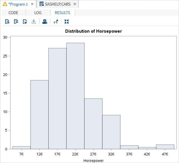
A elementary histogram is created by specifying the name of the variable and the range to be considered to group the values.

Example

In the below example, we consider the minimum and maximum values of the variable horsepower and take a range of 50. So the values course a group in steps of 50.

          proc univariate data = sashelp.cars;
histogram horsepower/ midpoints = 176 to 350 past l;
run;        

When we execute the in a higher place code, we become the following output −

SAS Histogram with Normal Curve

Let'southward start by creating a uncomplicated SAS histogram of the WEIGHT variable. We volition use the inbuilt information fix sashelp.course:

          Championship 'Summary of Weight Variable (in pounds)';
PROC UNIVARIATE Data = sashelp.class NOPRINT;
HISTOGRAM weight/NORMAL;
RUN;        

In the below example we fit a distribution bend with hateful and standard deviation values mentioned as EST. This option uses and estimate of the parameters.

Example :

proc univariate data = sashelp.cars noprint;
histogram horsepower/ normal (
mu = est
sigma = est
color = blue
w = 2.5
)
barlabel = percentage
midpoints = 70 to 550 past 50;
run;

When nosotros execute the above code, we go the following output −

2.Bar Nautical chart

A bar chart represents data in rectangular confined with length of the bar proportional to the value of the variable. SAS bar nautical chart shows the distribution of a chiselled variable. The bar nautical chart in SAS is some of the most commonly used graphs to convey information to the reader. Bar charts are used across all domains, including business, finance, banking, clinical and health, and life sciences.

SAS uses the procedure PROC SGPLOT to create bar charts. We can draw both simple and stacked confined in the bar nautical chart. In bar nautical chart each of the confined can be given different colors

Syntax

The basic syntax to create a bar-nautical chart in SAS is −

          PROC SGPLOT Information = DATASET;
VBAR variables;
RUN;            
QUIT;        

Following is the clarification of parameters used −

• DATASET − is the name of the dataset used.
• variables − are the values used to plot the histogram.

SAS Unproblematic Bar Chart

A elementary bar chart in SAS is the 1 that has single vertical bars. We have used the Olympics data prepare. This SAS Bar chart shows the number of countries in each region that participated in the 2022 Olympics.

          PROC SGPLOT Information = olympics;
VBAR Region;
Championship 'Olympic Countries by Region';
RUN;        

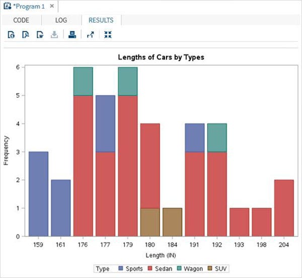
Stacked Bar chart

A stacked bar chart is a bar chart in which a variable from the dataset is calculated with respect to another variable.

The beneath script will create a stacked bar-chart where the length of the cars are calculated for each machine type. We utilize the group selection to specify the second variable.

Example

          proc SGPLOT data = work.cars1;
vbar length /group = type ;
title 'Lengths of Cars by Types';
run;
quit;        

When nosotros execute the above code, we get the following output

SAS Clustered Bar Chart

Like in the previous example the groups were stacked ane higher up the other, the variables can be stacked adjacent to each other that is side by side. Y'all tin specify side-by-side groups instead of stacked groups by adding the option GROUPDISPLAY = CLUSTER to the VBAR statement.

Instance

          PROC SGPLOT Data = olympics;
VBAR Region / GROUP = PopGroup GROUPDISPLAY = CLUSTER;
Title 'Olympic Countries by Region and Population Group';
RUN;        

3. Pie Nautical chart

A pie-chart is a representation of values as slices of a circle with dissimilar colors. The slices are labeled and the numbers respective to each slice is also represented in the nautical chart. SAS Pie Chart creates simple, grouping, or stacked charts that correspond the relative contribution of the parts to the whole by displaying data every bit slices of a pie. Each slice represents a category of data. The size of a piece represents the contribution of the data to the total chart statistic.

In SAS the pie nautical chart is created using PROC TEMPLATE which takes parameters to control percent, labels, color, title etc.

Syntax

The basic syntax to create a pie-nautical chart in SAS is −

          proc chart information= <dataset>;            
pie <variables>;            
run;            
/*or*/            
proc plot information= <dataset>;            
plot yaxis <variables> * xaxis<variables>/ <options>;            
quit;        

Following is the description of parameters used −

• variable is the value for which we create the pie chart.

The PIECHART performs detached binning for the CATEGORY column and calculates appropriate summarization statistics (sum, mean, and then on) based on the setting for the STAT=pick.

we can apply the START= and CATEGORYDIRECTION= options to control the pie slice positions and display order.

SAS Pie Charts with Data Labels

In this type of SAS pie chart, nosotros tin specify whether nosotros desire information values within the chart or exterior the chart. We can also represent value both equally a fraction every bit well as percentage. We then use options similar DATASKIN to modify the appearance of our chart.

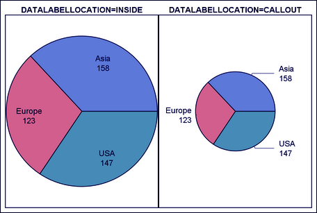
DATALABELLOCATION = AUTO | Inside | Exterior | CALLOUT
specifies whether to display the slice labels within the pie slices or outside of the pie circumference.

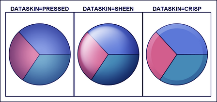
DATASKIN= NONE | PRESSED | SHEEN | CRISP | GLOSS | MATTE
enhances the visual appearance of the filled pie slices.

Grouped Pie Nautical chart

In this pie nautical chart the value of the variable presented in the graph is grouped with respect to another variable of the same data set up. Each group becomes one circle and the chart has as many concentric circles equally the number of groups available.

Example

In the below instance we group the chart with respect to the variable named 'Month'.

          goptions cback=black;            
pattern1 c=red;
pattern1 c=green; pattern1 c=yellow;            
proc gchart data=nutan.product_sales;            
pie3d prdcode/woutline=two coutline=white            
ctext=white explore='M6' group=month;            
Run;
Quit;        

when we execute the above code then we get the below output :

here is the another example :

In the below example we group the chart with respect to the variable named "Make". Equally there are two values bachelor ("Audi" and "BMW") and so we get two concentric circles each representing slices of motorcar types in its own make.

          proc gchart
PROC TEMPLATE;
DEFINE STATGRAPH pie;
BEGINGRAPH;
LAYOUT REGION;
PIECHART CATEGORY = type / Group = make
DATALABELLOCATION = INSIDE
DATALABELCONTENT = ALL
CATEGORYDIRECTION = CLOCKWISE
DATASKIN = SHEEN            
START = 180 NAME = 'pie';
DISCRETELEGEND 'pie' /
Championship = 'Car Types';
ENDLAYOUT;
ENDGRAPH;
END;
RUN;
PROC SGRENDER DATA = cars1
TEMPLATE = pie;
RUN;        

When we execute the above code, we go the following output :

iv. Scatter Plot

Scatterplot is a blazon of graph which uses values from two variables plotted in a Cartesian plane. It is usually used to find out the relationship between two variables.

A besprinkle plot in SAS Programming Linguistic communication is a type of plot, graph or a mathematical diagram that uses Cartesian coordinates to display values for two variables for a set of information.

Syntax

The bones syntax to create a scatter-plot in SAS is −

          PROC sgscatter  Information = DATASET;
PLOT VARIABLE_1 * VARIABLE_2/ datalabel = VARIABLE group = VARIABLE;
RUN;        

Following is the description of parameters used −

• DATASET is the name of data set.
• VARIABLE is the variable used from the dataset.

SAS Elementary Besprinkle Plot

In this blazon of SAS Scatter plot, two variables are selected and are grouped with respect to a 3rd variable.

          proc sgplot data=mylib.employee;
scatter 10=salbegin y=salary / group=gender;
run;        

SAS Scatter Plot with Prediction Ellipse

An ellipse approximates a region that contains 95% of the population. By default, the ellipse argument creates a prediction ellipse. The ellipse acts as an estimation parameter to predict the strength of correlation betwixt the two variables.

          proc sgplot data=sashelp.iris;
championship "Iris Petal Dimensions";
scatter ten=petallength y=petalwidth;
ellipse x=petallength y=petalwidth;
run;        

When nosotros execute the to a higher place code, nosotros get the following output −

Scatter Matrix in SAS

SAS Besprinkle Matrix consists of several pairwise besprinkle plots that are presented in the form of a matrix. The matrix tells us the correlation between unlike variables and whether they are positive or negative. They help us roughly determine if at that place is a correlation between multiple variables.

Instance

          proc sgscatter information=mylib.employee;
where jobcat=ane;
matrix salbegin salary jobtime prevexp / group=gender diagonal=(histogram kernel);
run;        

When we execute the to a higher place lawmaking, we go the following output −

5. Box Plot

A Boxplot is graphical representation of groups of numerical data through their quartiles. Box plots may too have lines extending vertically from the boxes (whiskers) indicating variability outside the upper and lower quartiles. The bottom and top of the box are always the get-go and 3rd quartiles, and the ring within the box is e'er the second quartile (the median). In SAS a simple Boxplot is created using PROC SGPLOT and paneled boxplot is created using PROC SGPANEL.

Simply, A box-and-whiskers plot displays the mean, quartiles, and minimum and maximum observations for a group.

Syntax

The basic syntax to create a boxplot in SAS is −

          PROC SGPLOT  Data = DATASET;
VBOX VARIABLE / category = VARIABLE;
RUN;                    PROC SGPANEL  Data = DATASET;
PANELBY VARIABLE;
VBOX VARIABLE> / category = VARIABLE;
RUN;        

Following is the description of parameters used −

• DATASET − is the name of the dataset used.
• VARIABLE − is the value used to plot the Boxplot.

Simple Boxplot

In a simple Boxplot we choose one variable from the data set and some other to grade a category. The values of the outset variable are categorized in as many number of groups as the number of singled-out values in the second variable.

SAS boxplot without any category:

          proc sgplot data=mylib.employee;
vbox salary;
RUN;        

A boxplot with the category:

          proc sgplot data=mylib.employee;
vbox salary/ category = gender;
run;        

SAS Boxplot in Vertical Panels

Boxplot in a group using some other tertiary variable which divides the graph into multiple panels. We tin divide the boxplots of a variable into many vertical panels(columns). Each console holds the box plots for all the chiselled variables.

          proc sgplot data=mylib.employee;
panelby jobcat/rows=1 columns=3;
vbox salary/category = gender;
run;        

SAS Boxplot in Horizontal Panels

This is very similar to vertical panels Boxplot. In this SAS boxplot, a variable is divided into rows. Like vertical, in this besides we categorize the information upon a tertiary variable.

          proc sgpanel information=sashelp.heart;
panelby sex/columns=1;
vbox bacon/category = gender;
hbox cholesterol/category=ageatstart;
title ' Cholestrol past Sexual practice and Age Grouping';
run;        

We can have more than than 1 analysis variable in the SAS Histogram statement. Each variable will have a divide histogram in SAS. NOPRINT option suppresses the summary statistics, the NORMAL option presents a normal curve.

References

1. Google
2. Tutorialspoimt
3. DataFlair
4. SAS Customs
5. PROC-X

Source: https://medium.com/swlh/sas-data-visualisation-9223dc30e039

Posted by: gonzalezaustens.blogspot.com

Share this post